
Hex-Based Terrain and Assisted Theory Crafting
as you may know i have been working on a game (github). it’s a philosophically-inclined hiking simulator where you go around and read stuff and talk to people and try to atone for something awful you did. i’ve been working on it for like 7 years now. but here’s something new: i’ve been using llms to speed up the process and boy HOWDY is it working wonders for me. let’s start by talking about the meat of what we’ve made before i start talking about llms and how i like to use them. if you’re annoyed by that part then just read the first half i don’t care
The design
As always, the design developed as I went along. The initial idea was to create a simple path-based hiking simulation over a terrain. Quell is meant to be about getting lost in the woods, atoning for something you did a long time ago. Nobody is apt to forgive you. And you have your own demons to deal with. It’s also about digital technology and the way it’s changed our lives.
The game has multiple loops. This initial loop, which is the game loop proper, is the hiking loop. Within that loop are several sub-games: discovering artifacts, reading and writing notes, using those notes and artifacts to talk to NPCs, and lore dumps which help the player proceed from hiking loop to hiking loop. Once certain conditions are met, the hiking loop starts over, regenerates the world, and the subgames are played again.
I wanted the player to come across several key locations, which I’ll call nodes. The spawn point is included in this set. Key locations include hollowed out old buildings, which the player will explore to find real philosophical texts. They’ll use these texts to talk with NPCs, who get their own nodes, to help them solve their problems. (The exact manner of this is to be decided.) And finally, there are flashback events. I’m torn between these happening randomly throughout the woods, triggered by certain conditions, or if they should be their own node type. Currently I’m working with the node type, since that’s just easier to implement. At these places, the player comes across scenarios from their past. In terms of the hiking loop, this scrambles the paths but leaves the nodes intact.
Initial experiments
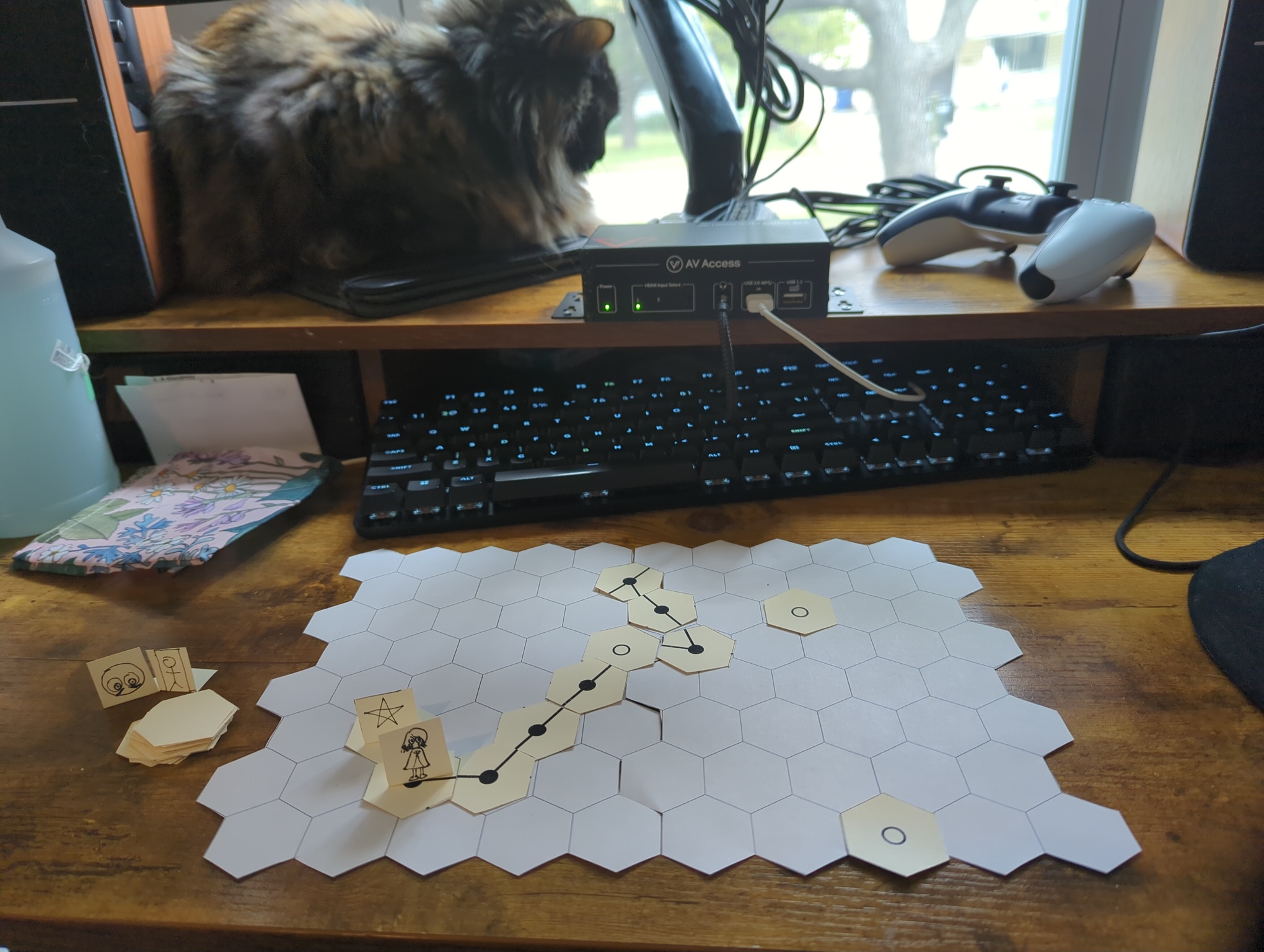
I started with an IRL prototype. My focus was on path routing and an abstract sense of exploration much more than terrain generation, so I used a simple hex grid for this. In the IRL prototype I had paths per-hex, with 2 or 3 spokes coming out the middle. Placing them in the middle instead of the edge is equivalent, just on the dual of the hex grid instead. This was easy enough to do. I had an agent print off some card stock with two copies of all of the possible two-spoke patterns and one copy of the three-spoke patterns, plus a small set of nodes with icons for points of interest. Then I added a standee for the player. POIs were placed in one deck, nodes in another. The board was set up with dice rolls on a hex grid; each node placement was determined by a dice roll (mod board size - which I now realize was probably the reason my nodes kept skewing to one side) for the x and y coordinates. The player would begin in the center of the board (or wherever else I wanted the spawn tile to go), and attempt to get to all the key points of interest. As the player proceeded, they would draw from the path deck and place down their tile, one at a time. This simulated path visibility, albeit somewhat crudely. While this wasn’t really how the end-result would be on the computer, it helped me think through the constraints I wanted for the paths and the various gameplay mechanics surrounding the nodes. Plus it was cool and fun to have physical artifacts.
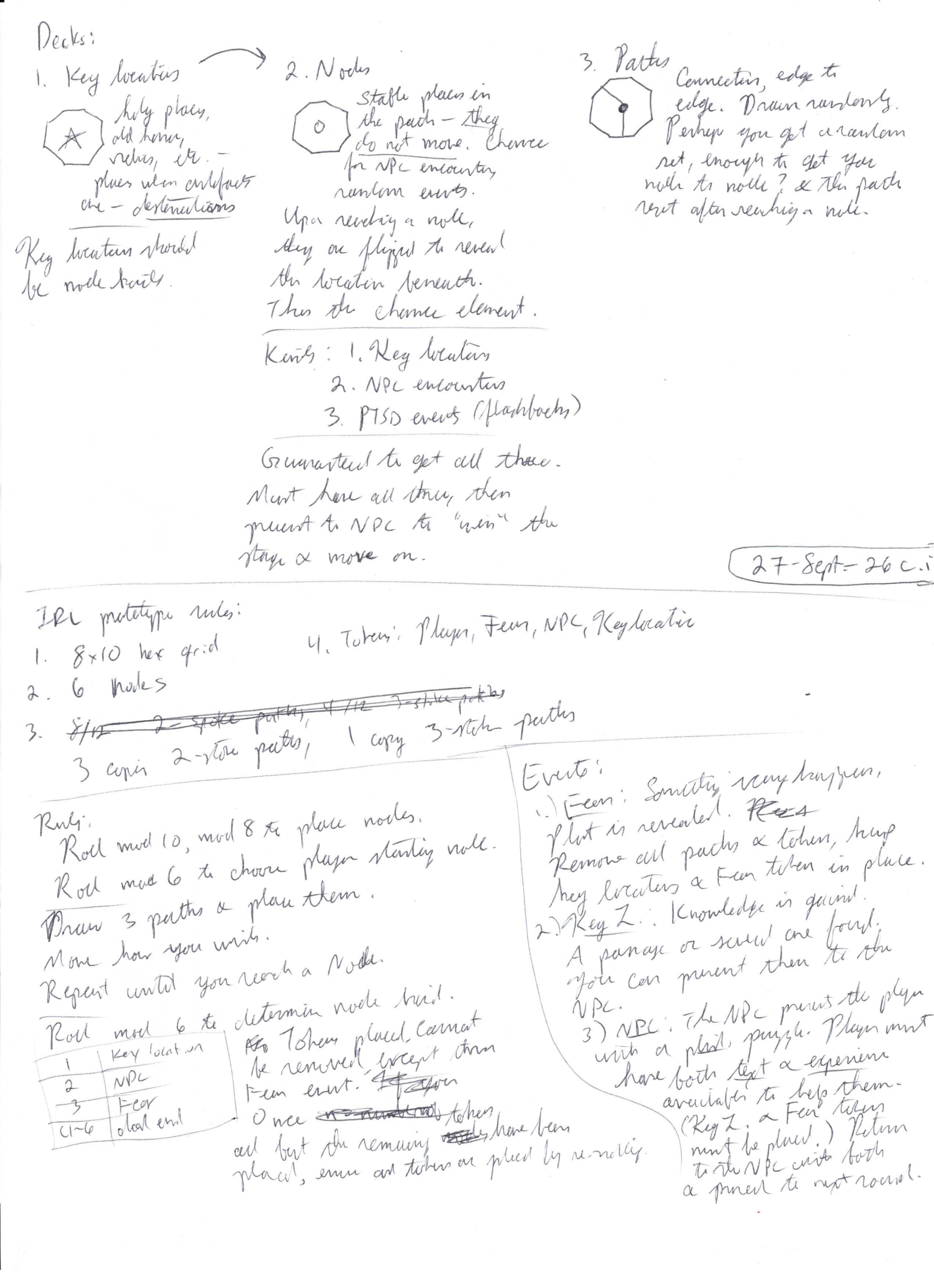
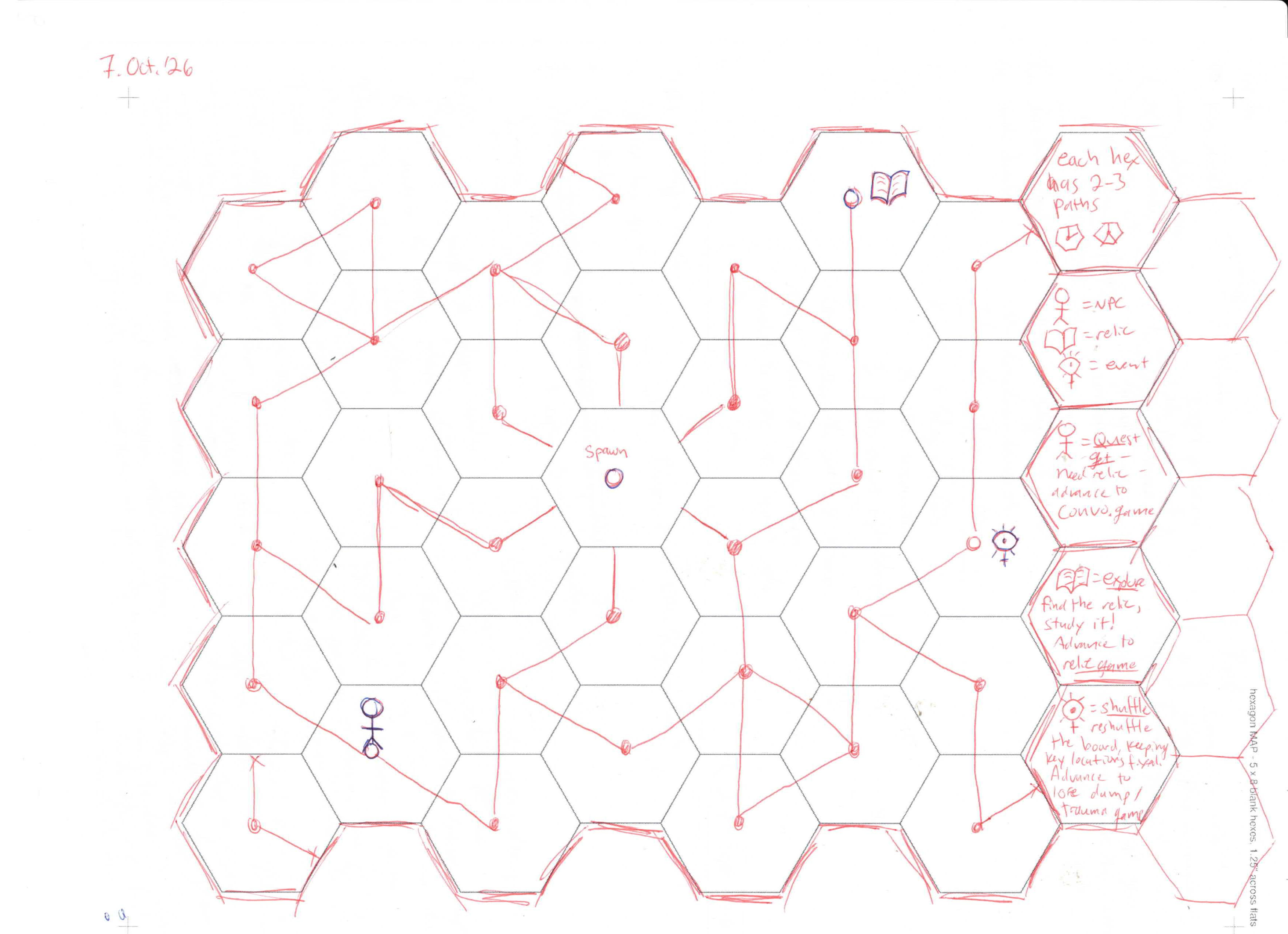
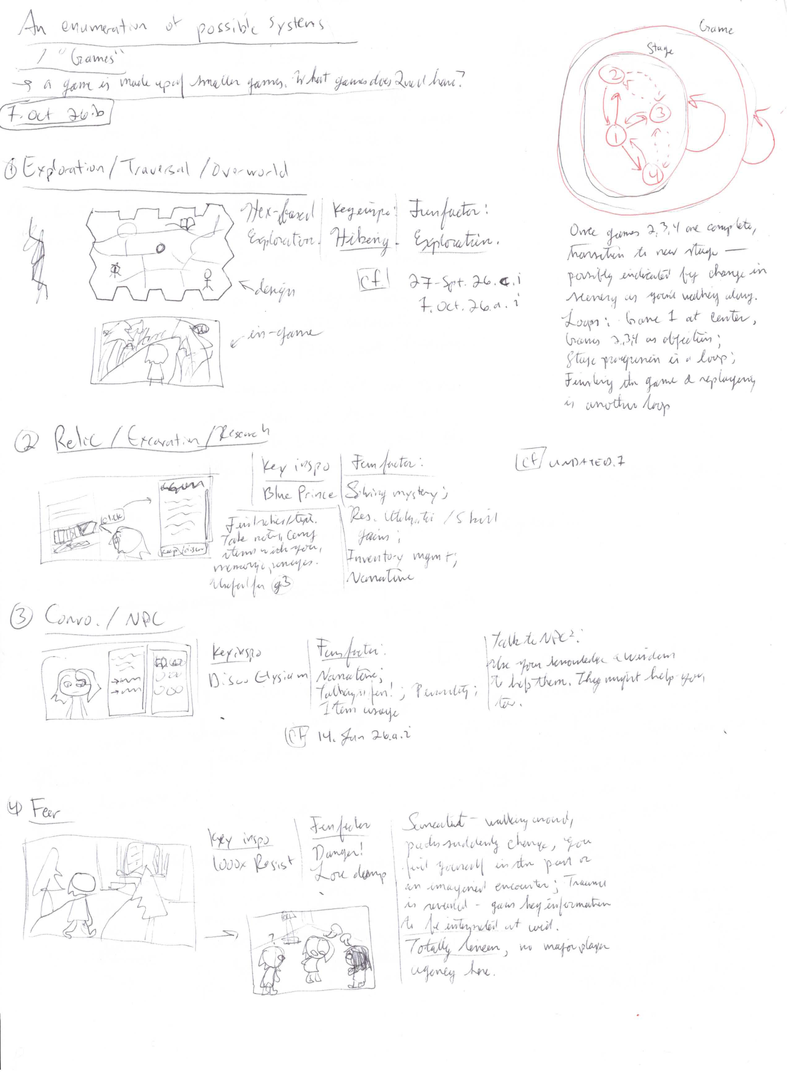
Next up was software. I scanned my sketches for the design and ensured the LLM understood what I had shown it. Then we discussed and came up with a design document, drafted to disk. Before hopping into implementation, we wrote out an attack plan, commit-by-commit. Issues were drafted from the plan, and implementation followed. I made sure we used existing libraries (like hexx and my own q_screens), with bevy_ui + bsn as the front-end for code tweaking. Settings were initially stored as resources, but I later converted these to assets to make tweaking easier. I used bevy_asset_loader to create asset collections and block on the load, and bevy_common_assets for RON serialization.
I started off just replicating the 2d board. It was a flat, gizmo-based hex grid with nodes, paths on the edges. From there we started experimenting with rules for node placements and path constraints. Originally, we were just playing around with pathfinding algorithms. Then I realized that we were going about it backwards – instead of building the terrain around the paths, we need to build the paths around the terrain. This is obvious in hindsight, but moving from 2d to 3d it wasn’t immediate :)
I had the bots whip up a python laboratory to do some quick experiments over large sample sizes for the different path algorithms. We were trying to restrict the number of path tiles, loops, and other such path properties directly as a factor of the algorithm. Here are some of the visuals we got out of it.
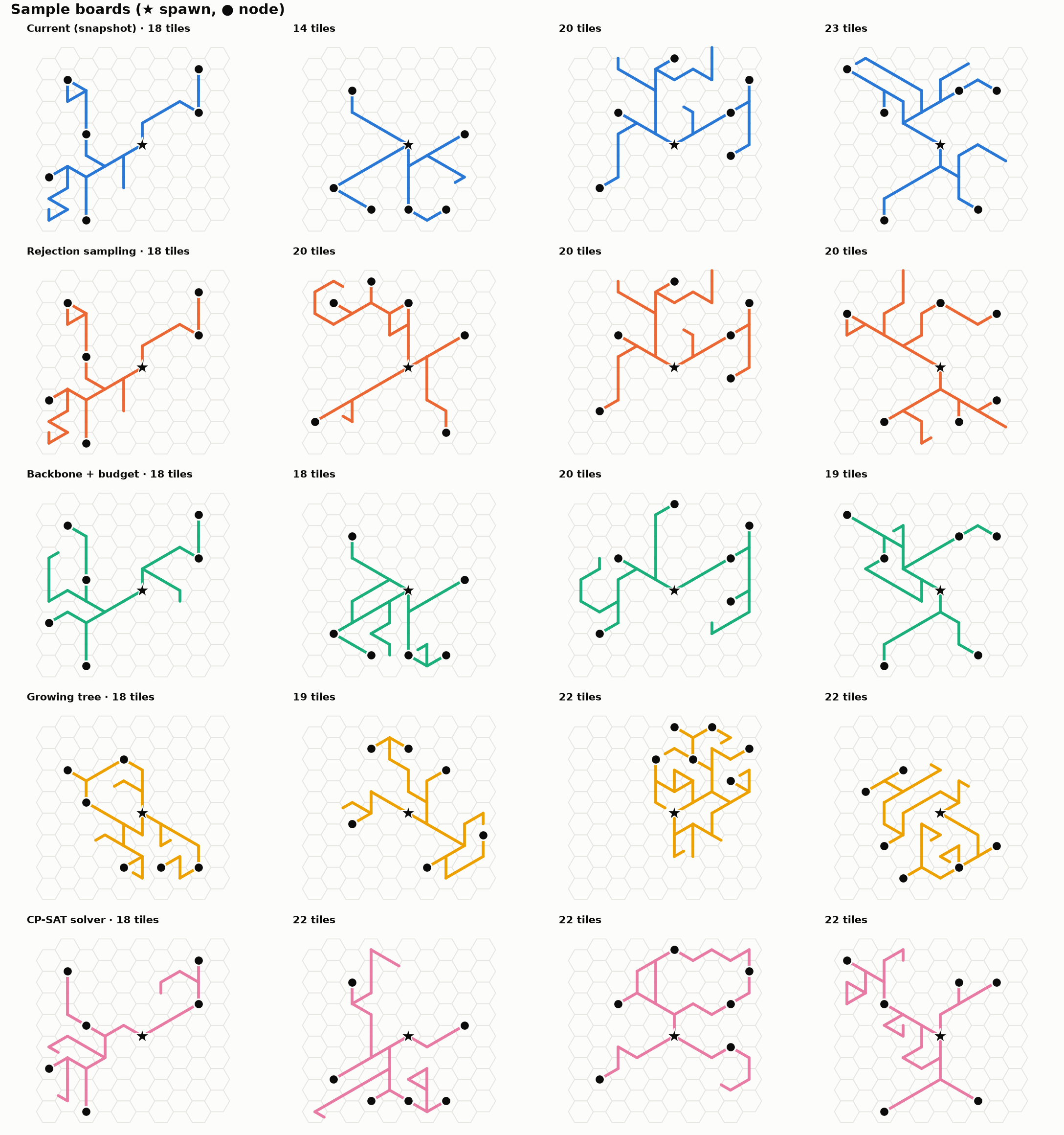
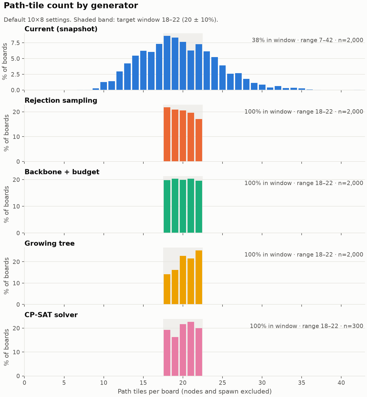
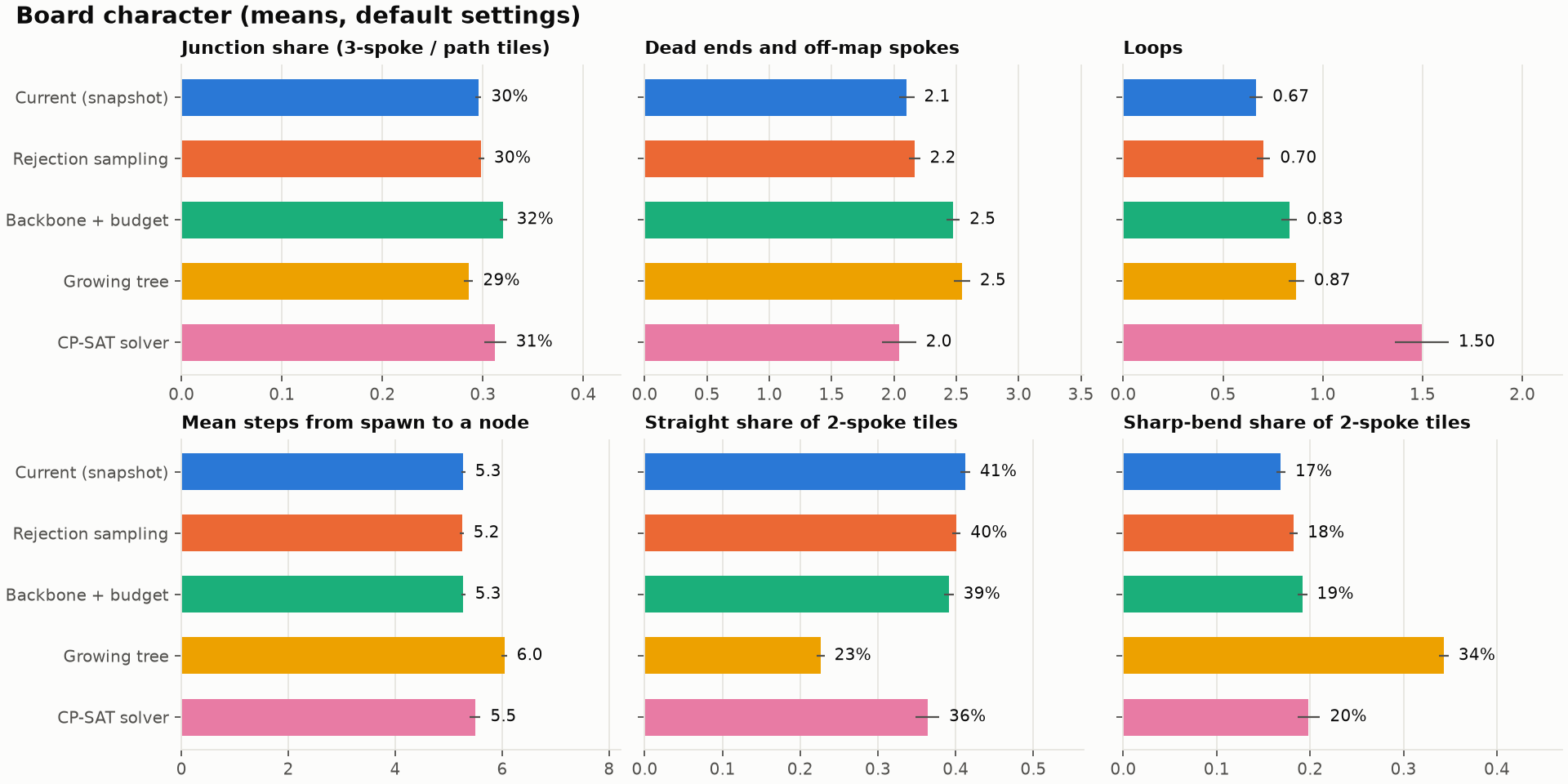
We didn’t begin moving back to rust for a bit as the python code was faster to iterate with and we could still visualize everything in 2d using SVG-based visualizations for a heightmap, color-coded for height like a typical geographical survey. We began with a typical perlin noise based terrain algorithm. From there we added tweaks. I’m basing this game off of hikes I’ve been on, in the glacial hills of northeast Kansas, so we landed on rolling hills and creeks cutting into the loam, oak and hickory dense around the water.
In order to make a path, we need to rank how easy it is to hike around. So we used a symmetric approximation of the Tobler hiking function to rank edges. From there, we place the nodes according to suitability and link between them using a slightly noisy A* algorithm.
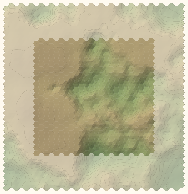
Figure 12: Terrain 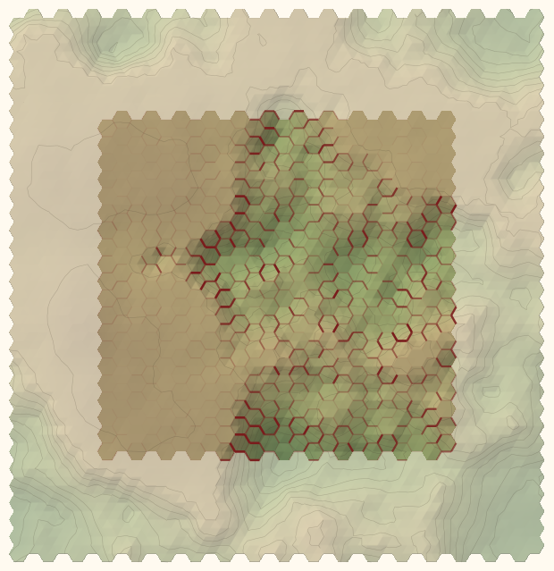
Figure 13: Path cost 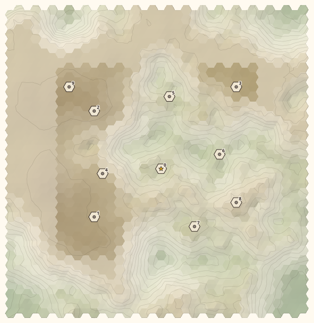
Figure 14: Node placement 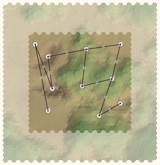
Figure 15: Connected node network, ranked by cost 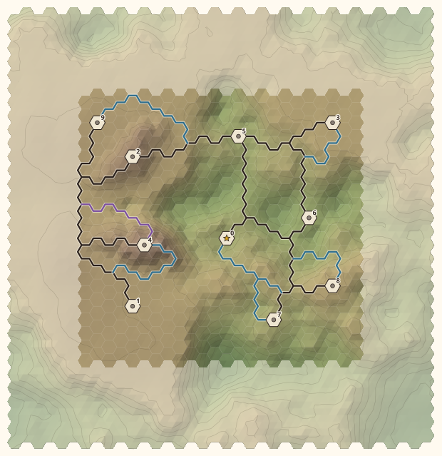
Figure 16: Path placement
We limit paths by a budget over edge weights. In Figure 15 above, note that nodes 0 and 2 do not even have a candidate connection as the cost between them would be too high. Paths are chosen based on a greedy graph spanner, weighted by various factors such as hiking cost, whether they make a loop between nodes, and whether they create a ‘tease’ between two nodes. We’ll discuss this more below. Extra pathing is added after the initial greedy spanner as necessary to maximize the constraint score.
Formalizing the generation method
This is the part where it gets mathy. I decided to write out the ontological bits in mathematical notation because it’s easier to express objects that way, while procedural bits are written in a rusty pseudocode. Feel free to skim this section if the gory details aren’t of interest to you.
Points of Interest
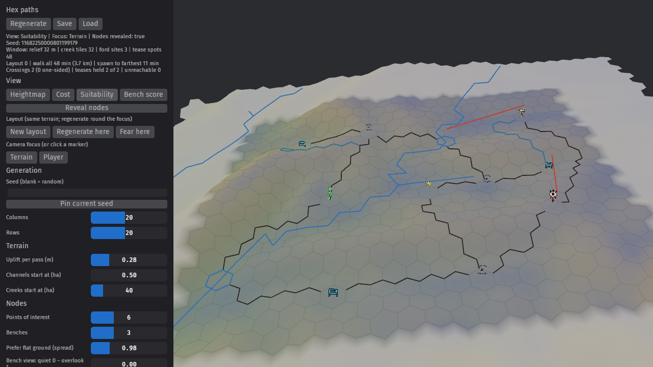
Let’s define the board as the set of all playable tiles. Note that this is a window over a larger hex grid which I’ll call the world grid, . The size of the world grid is parameterized by the column and row layout plus a padding radius which I’ll denote here as .
Let denote the height of a vertex , and let be the set of six corner vertices of a hex tile . Let be T’s neighborhood tiles. Our board is a window over a larger hex grid, so all tiles are interior. Note that . The height range over that neighborhood is
Let be the median range over the board, . Then we define the suitability score as
Perfectly flat ground scores 1, and a tile exactly as bumpy as the median tile scores . Because the range is divided by the median, “flat” is relative to the board, so on bumpy boards the flattest available ground still scores well.
Next, introduce , our spread variable. Raising suitability to the power sharpens it: the larger is, the more strongly POIs prefer the flattest ground. At flatness is ignored entirely. On bumpy terrain, flat patches are scattered, so POIs end up scattered too; on a plateau, they gather towards it.
People naturally build structures towards water, so let’s define a constant to track this. The larger is, the more POIs favor ground near water. Let be the set of creek tiles, and let be the distance from to the nearest creek tile, measured in hexes. The water pull factor is
so a tile right beside a creek gets up to times the weight, fading over a couple of hexes. Nothing but a crossing may sit on a creek, so the final placement weight is
Placement doesn’t sample tiles in proportion to . Instead, each POI goes on the tile that best balances weight against distance from everything already placed.
fn place_poi(board: &Board, placed: &[Tile], rng: &mut Rng) -> Tile {
    board.tiles()
        .filter(|t| !placed.contains(t))
        .max_by_key(|&t| {
            // Distance to the nearest placed node; the board's edge counts
            // too, but repels only half as strongly.
            let separation = placed.iter()
                .map(|&p| hex_distance(t, p))
                .fold(2.0 * edge_distance(t), f32::min);
            separation * w_p(t) * rng.jitter()
        })
}
Benches
When you’re on the trail, you need to take a break every now and again. Maybe you need to reorganize your stuff or you just need a breather. Benches offer that. I want to place them somewhere with a sense of beauty. There are two really contemplative views, I think: those with a great view, like a mountain-top, or those tucked away in a dense patch of green. Both are questions about what you can see from a tile, so let’s put a viewer on every tile and look around.
Let be the center of tile , and let be the ground height at any point on the terrain - on or off the lattice. Our viewer’s eye sits a height above the ground, and they look at every other tile within a radius of hexes. We’ll define the set of tiles within that radius as follows:
The converts hexes to edge lengths, since neighboring tile centers are edges apart.
Let be the tiles we can see – namely, those where a ray from the viewer’s eye at to the ground at isn’t blocked by the terrain. We check this with a simple ray march, sampling points along the way.
We can get two measures from this. The first is openness: the ratio of visible tiles over the given radius.
But for nooks, what we’re looking for is the opposite of openness. So let’s just take the complement:
Our second score is for dramatic views. Let the parameter denote a height saturation point. Anything bigger is capped. With a small , almost any visible height difference counts fully, so we’re mostly counting how many tiles differ from us. With a large , few differences reach the cap, so dramatic cliffs and deep gullies win.
Set , positive when is below us. Define as a parameter weighing upward views against downward ones. We can then define a tweakable measure for finding high-relief (dramatic) bench placement scores.
The caps each tile’s contribution at 1, so each tile’s score is normalized. This makes , which maximizes to a range of .
Note that we divide by , not . We want to measure the proportion of high-relief tiles that are visible within a certain radius, so we sum over those visible tiles and divide over the total. This way a spot that sees only a sliver of a big drop scores less than one that sees the whole valley.
So we have our two bench scores, quiet and relief. But their distributions aren’t normalized. So let’s normalize them. For a score ,
so that and are both . Once we’ve normalized them into proper ranks, we can sort them. Ranks only care about order, so a board with a few dramatic cliffs and a board with gentle hills both get their best spots ranked at the top.
But let’s suppose there are few good spots. We should introduce a sharpness parameter to reduce the likelihood that a boring location is picked. Let be that parameter. Raising a rank to the power crushes everything except the very top, so only the most enclosed spots and the best views score well. Ground that’s middling at both doesn’t win.
We also want to control whether benches get placed in quiet spots or at dramatic overhangs. Set as our view preference, from 0 (quiet benches) to 1 (dramatic benches). Now we can define our final bench weight function:
Benches are placed the same way as POIs, using instead of . Like POIs, they stay off creeks, and they try to keep a minimum distance from one another.
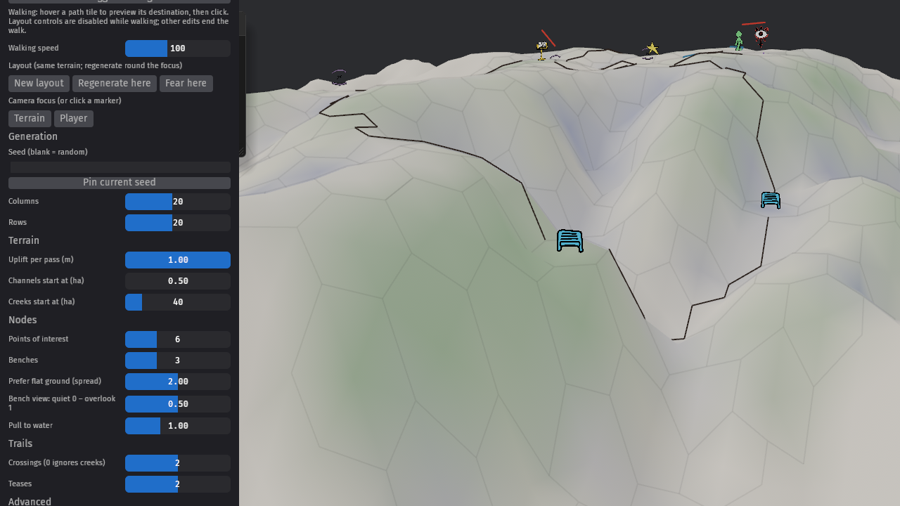
Figure 19: A dramatic bench 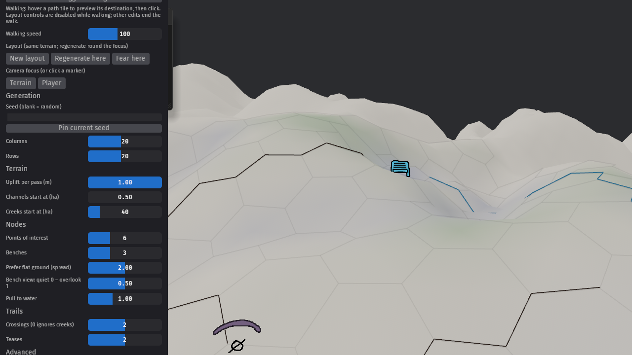
Figure 20: A (relatively) quiet bench
The quiet benches don’t look so quiet here, but you have to imagine them surrounded by forestry. We’re early in development, so a little imagination goes a long way :)
Trails
Cost
Now that we’ve placed the nodes, we need to join them. Our terrain is a large hexagonal lattice, but here we’ll need to represent it as a graph. I use a calligraphic font here to make the relationship between the hex sets and the graphs apparent.
Let’s write the edges of a graph as , sim. for vertices, so that . The playable board is a window over this larger terrain, so let’s define that as . Now, let’s call the set of edges which a creek crosses. Note that while the correspondence between and is a direct translation from set to graph, does not relate to any particular graph, but only to a subset of the edges defined in above.
Let denote all nodes. The subset contains all POIs. Each node sits on flattened out ground. Its tile is leveled and the ground around it graded to match, so we can easily fit pre-authored scenes onto it. Let be the height of vertex after leveling.
Walking uphill or downhill is harder than walking on the flat, so the cost of an edge grows exponentially with how much it climbs. Let be our aversion to slopes, and let denote the set of all paths over . Then we can define as the weight for an edge .
We obviously don’t want paths to lead straight into a creek or off the board, so we denote this by setting the cost to infinity.
is our symmetric Tobler approximation; the original gives a walking speed in km/h: .
Let’s denote the paths from nodes to as . For any edge weighting and nodes , let’s write to denote the least expensive path from to given some weighting .
So, is the least expensive path weighed by the cost of walking cross-country. The same formula can be used for other The most efficient method of selecting a trail path would be to select the least expensive route. But efficiency isn’t fun, so that’s not what we do. We’ll define exactly how we differ from the optimum below.
As we lay trails, let be the set of laid edges. We want to know how far the walk is if we stick to the trails. The cost of walking across an edge is defined below. Note that we let paths cross nodes for free.
We can use this to measure how far off the ideal geometric path we are. By the path cost function above, the cost is always nonzero except across nodes, so we almost never take the ideal path. We can use the ratio to measure how far off the preferred path we are.
The spanner
We don’t want trails to be too long. Getting lost is a big part of the game, so we need lots of branching paths and opportunities for decision making. We can accomplish this by using a graph spanner. In particular, we use a greedy spanner.
Start by calculating over . Then sort by value, starting with the lowest cost. For each pair, check whether the network already gives a reasonable walk. Define a parameter for the spanner’s stretch; if the walk is more than times the cross-country cost we lay a new trail. This way we add just enough trail that no node is more than times worse off than walking straight there. We additionally use a final pass to ensure that every node can be reached from spawn.
New trails should merge into old ones rather than run beside them, so routes are planned with two adjustments to the cost: a discount for reusing trail, and a penalty for walking alongside a trail without joining it. “Alongside” means a band of edges just off the trail:
/// Penalise edges that run beside a trail without joining it.
fn alongside(trail: &Trail, radius: u32) -> impl Fn(Edge) -> f32 {
    // How many hops each corner is from the trail, out to `radius`.
    let hops = breadth_first(trail.corners(), radius);
    move |(u, v)| {
        let on = |c| trail.touches(c);
        let near = |c| hops.contains(c) && !on(c);
        // Stepping onto the trail is never penalised.
        if !on(u) && !on(v) && (near(u) || near(v)) { GAMMA } else { 1.0 }
    }
}

/// Greedy spanner over the graph
fn span(nodes: &[Node], trail: &mut Trail) {
    let mut pairs: Vec<_> = node_pairs(nodes)
        .filter(|&(a, b)| !trail.is_tease(a, b))
        .collect();
    pairs.sort_by_key(|&(a, b)| d(cost, a, b));
    // Twice: a pair the tease guard rejects early may pass later.
    for &(a, b) in pairs.iter().chain(&pairs) {
        if d(trail.network(), a, b) <= T * d(cost, a, b) {
            continue; // already a reasonable walk
        }
        let beside = alongside(trail, 1);
        let reuse = |e| if trail.contains(e) { ZETA } else { 1.0 };
        let weight = |e| cost(e) * reuse(e) * beside(e);
        trail.lay_guarded(&[cheapest_route(weight, a, b)]);
    }
    // Anything still cut off joins the nearest node we can reach.
    while let Some(a) = trail.nearest_cut_off(nodes) {
        let routes = cheapest_routes(cost, a, trail.reached()).take(40);
        if !trail.lay_guarded(&routes) {
            trail.lay_unguarded(&routes[0]); // may break a tease
        }
    }
}
Loops
A spanner is a tree-like thing, full of dead ends, and dead ends make for frustrating hikes. So every node that isn’t already on a loop gets a second way out. A node is on a loop when there are two paths from it to another node that share no vertices along the way.
Let’s define a few new parameters. Each new loop should be comparatively cheap, a factor cheaper than the node’s existing link. The new edge should be at most edges long, and make a round trip of at least edges, so it doesn’t just circle the pad.
fn close_loops(nodes: &[Node], trail: &mut Trail, limits: Option<Limits>) {
    for n in nodes {
        if trail.on_loop(n) {
            continue;
        }
        // No reusing trail, and keep clear of the branch n hangs from,
        // so the loop isn't a thin finger running alongside it.
        let beside = alongside(trail, 2);
        let weight = |e| {
            if trail.contains(e) || near_own_branch(trail, n, e) {
                f32::INFINITY
            } else {
                cost(e) * beside(e)
            }
        };
        let budget = KAPPA * trail.nearest_link(n);
        let routes = cheapest_routes(weight, n, trail.other_trails_and_pads(n))
            .filter(|pi| pi.len() + trail.back(n, pi) >= LAMBDA)
            .filter(|pi| limits.is_none_or(|_| pi.cost(weight) <= budget && pi.len() <= XI))
            .take(40);
        trail.lay_guarded(&routes);
    }
}

close_loops(&nodes, &mut trail, Some(limits)); // cheap loops
close_loops(&nodes, &mut trail, None);         // second chance, no limits
Here back(n, pi) is how many edges it takes to walk from where joins the network back to .
Teases
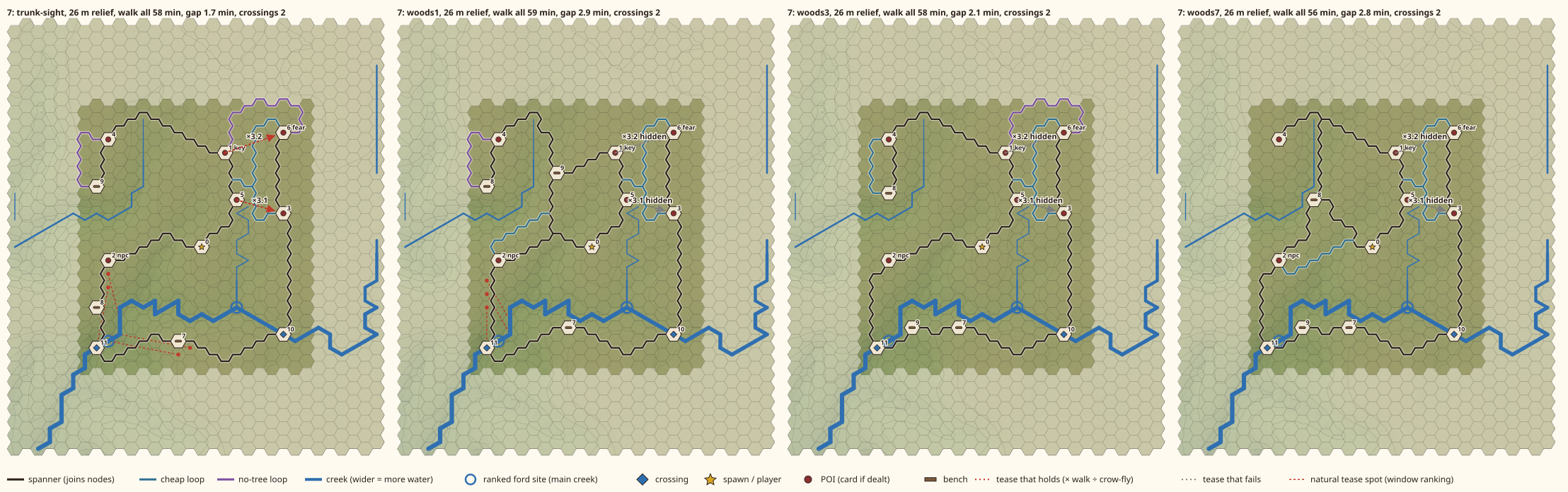
A tease is a view of something you can’t easily reach: you see a point of interest from a viewpoint, but the trail makes you take the long way round.
Let be the number of trail edges between two nodes, and how far a node is from spawn. Consider a viewpoint node and a target node . can be a tease if is a POI (not a bench), it’s within sight at , and . This way a tease always targets a POI, ensures that POI is visible, and ensures that the tease is earlier on the trail than the target.
fn choose_teases(nodes: &[Node], walked: &Walked, count: usize) -> Vec<(Node, Node)> {
    let mut candidates: Vec<_> = node_pairs(nodes)
        .filter(|&(v, t)| t.is_poi() && crow(v, t) <= SIGHT && walked[v] < walked[t])
        .collect();
    // Visible pairs first, then the biggest drops, then the closest.
    candidates.sort_by_key(|&(v, t)| (!visible(v, t), -drop(v, t).min(TOP), crow(v, t)));
    let mut used = Set::new();
    let mut teases = vec![];
    for (v, t) in candidates {
        if teases.len() == count {
            break;
        }
        if !used.contains(v) && !used.contains(t) {
            teases.push((v, t));
            used.extend([v, t]);
        }
    }
    teases
}
A tease only works if the walk from to is a real detour. Let be the minimum detour length in edges. We compare the walk with the open ground between the two nodes, which we define as the center-to-center distance minus a radius at each end:
A tease is broken iff the detour is too short, or if the player could reach the target before the viewpoint. Namely, if or .
Let be the set of broken teases for trail network . Once we lay the spanner, we want to guard our teases. A new route is only accepted if it doesn’t break anything that wasn’t already broken, that is if the following invariant holds: .
Sometimes a node can only be connected by breaking a tease. When that happens, we give up on that tease and lay the trail anyway (it shows in magenta). We then rebuild the whole layout so another tease can take its place.
fn generate(seed: u64) -> Layout {
    // A first build without teases tells us the order the player meets nodes.
    let walked = build(seed, &[]).walked_from_spawn();
    let mut disqualified = Set::new();
    let mut layout = None;
    for _ in 0..RETRIES {
        let teases = choose_teases_except(&walked, &disqualified);
        let attempt = build(seed, &teases);
        if attempt.broken().is_empty() {
            return attempt;
        }
        disqualified.extend(attempt.broken());
        layout = Some(attempt);
    }
    layout.unwrap().without_broken_teases()
}

fn build(seed: u64, teases: &[(Node, Node)]) -> Layout {
    let nodes = place_nodes(seed);
    let mut trail = Trail::guarding(teases);
    span(&nodes, &mut trail);
    close_loops(&nodes, &mut trail, Some(limits));
    close_loops(&nodes, &mut trail, None);
    join_creek_banks(&nodes, &mut trail);
    Layout::new(nodes, trail)
}
Reflections on Method
Grant Sanderson of 3Blue1Brown recently put out a video on the recent advances of AI models in mathematics. In it, he proposes writing proofs, asking questions, theory building, and applying theory as the key aspects of mathematics. For me, this is quite similar to what happens in philosophy. Around 20:00, he discusses the impact it would have in the world of mathematics if AI becomes better than humans at proving theorems. And essentially, he claims it has no impact on the overall structure and institution of mathematics, but it would change the culture from one of number-crunching to one of theory crafting.
What does the practice of doing math actually look like if the machines are better at the proof generation? Well, if we take that optimist’s perspective, the one who’s exhilarated by it, it basically looks like leaning into the theory building. You are no longer rate limited by how quickly you can solve certain problems along the way. You can ask all of the questions that you want. You can much more quickly see what the solutions to them are. You can try to parse that and just understand how does this fit into a bigger narrative. What are the elements of simplicity among all of the proofs that I’m looking at? And how can I weave this together into a fabric of a new kind of theory[?]
To me, this is an incredibly exciting development. AI has made me orders of magnitude more productive, and has enabled me to do the very theory-crafting he proposes. Except, in my case, the theory is not about numerical systems but about game design and the engineering that goes into it.
I can focus more on design in all aspects. Instead of spending a month struggling to find resources on game development e.g. how rasterization over a terrain mesh works, or how path finding algos work and how to tweak them, i can prompt to ask and it teaches me at a high level, then implements it. i may not have the hard-earned experience of crunching the numbers myself, but for game design that was never the point.
I don’t have to re-do solved problems. The knowledge I need isn’t expert-level and in depth – i need know how not know that – these algorithms are tools, not the object of my art. Obviously this isn’t to say that an algorithm cannot be its own aesthetic object, lest the lobsters have my head. But for me, as a game developer, what I need is a repertoire of common algorithms and the ability to use them in a practical manner. Reinventing the wheel will get me stuck at the engine level – which is a lovely place to be! But I’m ready to move on and actually make something. My focus has gone from attempting to match the standard to using the standard as a tool to achieve my own local vision.
An algorithm is like a ball bearing. It can be a beautiful thing! But most of the time you don’t care about how it works, just that it works, and in what situations it is useful.
Having these tools ready at my fingertips makes spiking incredibly easy. The hex terrain was initially tested in a python lab for quick compilation and turnaround. we did statistical analysis over 1000 seeds per run, generated SVG-based visualizations for the terrain, and several graphs tracking things like path loop count, bench locations, creek depth, and time to cross all paths based on the Tobler hiking function. It would have taken me a month or longer of full time work and research to do this on my own. I spent 3 days on it.
The primary lesson I want to put out here though is that one needs to be responsible for the code that their agents are producing. They’re automation machines, which makes code review extremely important. And code review is not that hard! It’s a bit boring, yes, but it’s worthwhile to understand what you’re producing. And yes this leads to fatigue, but so does coding. Having somewhat messy code for the sake of moving on is super common, especially in long-term projects. It can always be cleaned up later if needed. Spending all your time polishing a single algorithm is pointless if that algorithm is a part of something much larger.
The output of an agent doesn’t have to be slop. It’s not if you review, if you have proper ownership and safeguards. Agents can be coaxed into producing really good output very quickly, but you have to know how to tune it to your specifications. It may not always be organized exactly how you like it, or produce exactly what you would have, but you can work around that. I have file organization in my AGENTS.md and reinforce it at review time.
Speaking of review, automated review with a subagent is extremely important for catching subtle bugs. But it’s also important to know what’s worth doing now and what’s a red herring. These machines are meant to provide you the highest quality code, but are trained on a huge corpus of code – that means they’ll often write middling code and point out nits that don’t matter. It takes discipline and skill to know what’s worth doing. in the end, you are still the operator and you still own the output. Act like it!
—
so in summary: we made a sick little terrain generation thingy, and it happened very quickly and with very good results. this was the outcome of $20/month of tokens over the course of about two weeks. This would have taken far more than double the time doing it by hand. In terms of pure efficacy there is no question that this is the way I have to work if I want to achieve my ambitions. Whether it is ethical to do is another question, one I’ve explored elsewhere. But for now, because I need a job and I will probably kill myself if I don’t make this game soon, I am going to be using the bots. I would prefer to be doing it locally. Let’s hope I get a job soon so I can get a GPU and stop relying on massive amounts of cloud compute.